
20 LeetCode Patterns Every New Grad Must Know Before Interviewing at FAANG (2026)
A complete reference of the algorithmic patterns that recur in current FAANG coding interviews. What each pattern is, when it shows up, and the signal that tells you to reach for it.


FAANG coding interviews are not random.
The space of possible problems looks infinite from the outside, but the actual patterns recur.
A new grad who recognizes that a problem is a sliding-window problem within the first minute can solve it.
A new grad who tries to solve it from scratch without recognizing the pattern usually cannot, regardless of how smart they are.
This is the reference for the 20 patterns that cover the overwhelming majority of new grad FAANG coding interview problems in 2026.
The patterns are not new. They have been the foundation of coding interviews for over a decade.
What changes year to year is which patterns are most common, what the problem statements look like, and which combinations appear together.
The patterns themselves are stable.
This post lists all 20, with a definition, the signal in problem statements that tells you to reach for the pattern, one canonical example, and what the pattern is actually testing.
How to Read This Reference
The 20 patterns are organized into four tiers based on frequency in new grad FAANG interviews.
Tier 1 (the top 5) appear in nearly every new grad coding loop.
Tier 4 (the bottom 5) appear less frequently but are recognized as standard patterns that strong candidates know.
If you have limited time, work the tiers in order.
Tier 1 alone covers roughly 50% of the problems you will encounter. All four tiers together cover roughly 95%.
For each pattern, the most important section is “the signal.” That is the specific phrase or constraint in a problem statement that tells you the pattern applies.
Strong candidates recognize patterns from problem signals within 60 to 90 seconds, which is what allows them to solve under interview time pressure.
TIER 1: The Top 5 (Appear in Nearly Every Loop)
Pattern 1: Two Pointers
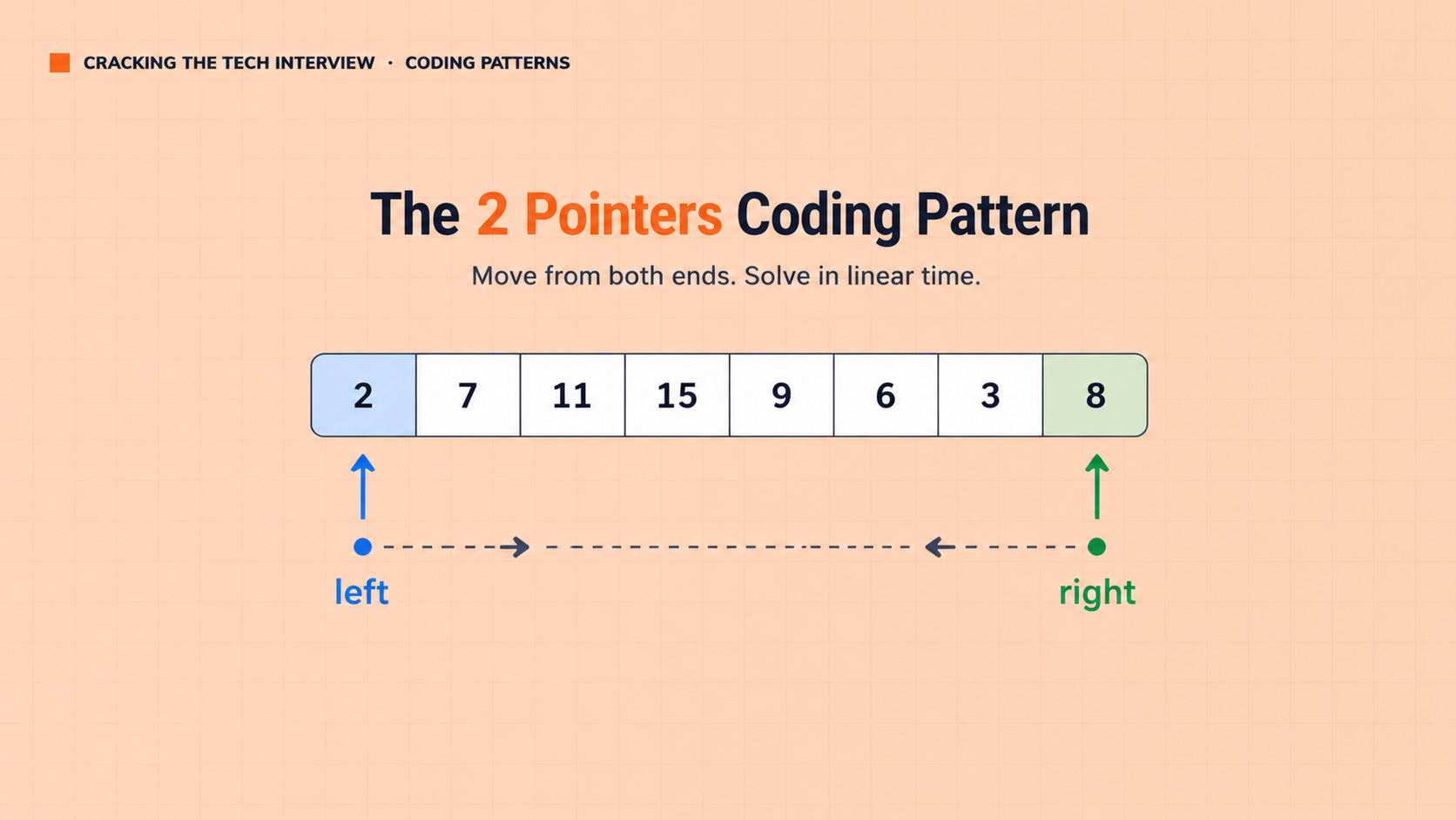
What it is: Use two indices that move through an array or string, usually toward each other or in the same direction, to solve problems in O(n) time that would otherwise be O(n²).
The signal: Sorted array. Pairs or triplets. Comparing two ends of a sequence. Words like “sorted,” “pair,” “find two,” “palindrome,” “container.”
Canonical example: Given a sorted array, find two numbers that sum to a target. Place one pointer at the start, one at the end. If sum is too large, move right pointer left. If too small, move left pointer right.
What it tests: Whether you recognize that ordered data unlocks an O(n) approach instead of the O(n²) brute force.
Pattern 2: Sliding Window
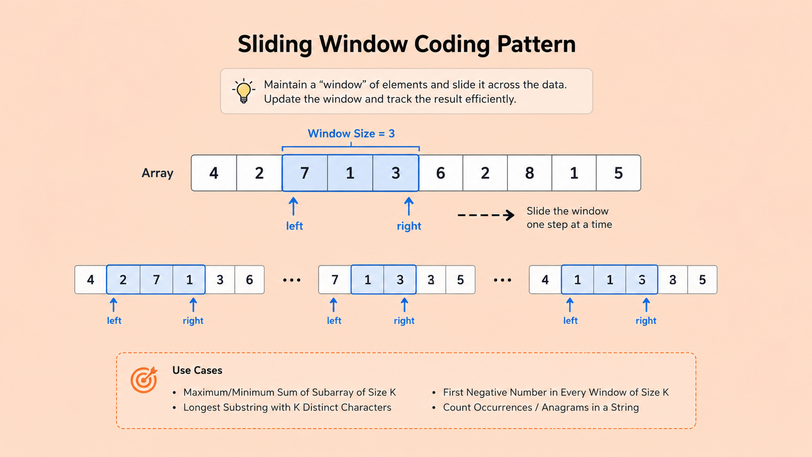
What it is: Maintain a window over a contiguous subarray or substring, expanding from one side and contracting from the other based on whether the window satisfies a condition.
The signal: “Contiguous” subarray or substring. Words like “longest,” “shortest,” “smallest,” “largest” combined with “window” or “subarray” or “substring.” Constraints like “at most K distinct” or “no repeating.”
Canonical example: Find the longest substring with no repeating characters. Maintain a window with a hash set tracking characters in it. Expand from right, contract from left when you hit a duplicate.
What it tests: Whether you can convert a contiguous-subarray search from O(n²) to O(n) by reusing state.
Pattern 3: Hash Map / Hash Set Lookup
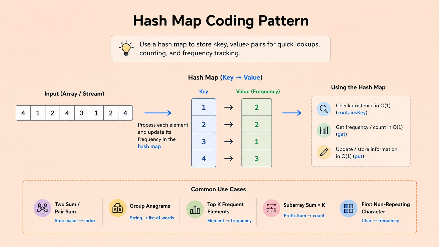
What it is: Use a hash table to convert what would be an O(n²) search into O(n) by precomputing or caching values.
The signal: “Have I seen this before.” Counting frequency. Finding a complement. Words like “count,” “frequency,” “duplicate,” “first occurrence.”
Canonical example: Two Sum (unsorted). For each element, check if its complement is in a hash set. If yes, return the pair. If no, add the current element to the set.
What it tests: The reflex to convert any “have I seen” or “is this in here” question into O(1) lookup.
Pattern 4: Binary Search
What it is: Repeatedly halve the search space by checking the middle element and discarding the half that cannot contain the answer.
The signal: Sorted input. Or any monotonic property. Words like “sorted,” “find,” “minimum that satisfies,” “Kth smallest.” Also: any problem where you can binary search the answer (the answer space is bounded and you can check feasibility for any candidate value).
Canonical example: Find an element in a sorted array. Standard binary search. O(log n).
What it tests: Whether you can recognize when O(n) can be reduced to O(log n) through the divide-and-search structure.
Pattern 5: Tree Traversal (DFS and BFS)
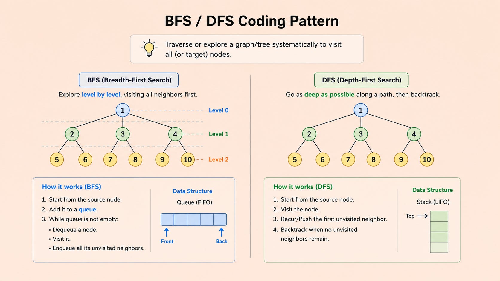
What it is: Walk through a tree or graph using either depth-first search (recursive or stack-based) or breadth-first search (queue-based).
The signal: The problem involves a tree, a graph, or any hierarchical/connected structure. Words like “tree,” “graph,” “ancestors,” “level,” “shortest path.”
Canonical example: Maximum depth of a binary tree. Recursive DFS. For each node, return 1 + max(depth of left, depth of right).
What it tests: Foundational graph and tree traversal. New grads who cannot do this fluently fail at every FAANG.
TIER 2: The Next 5 (Appear Frequently)
Pattern 6: Dynamic Programming (Basic)
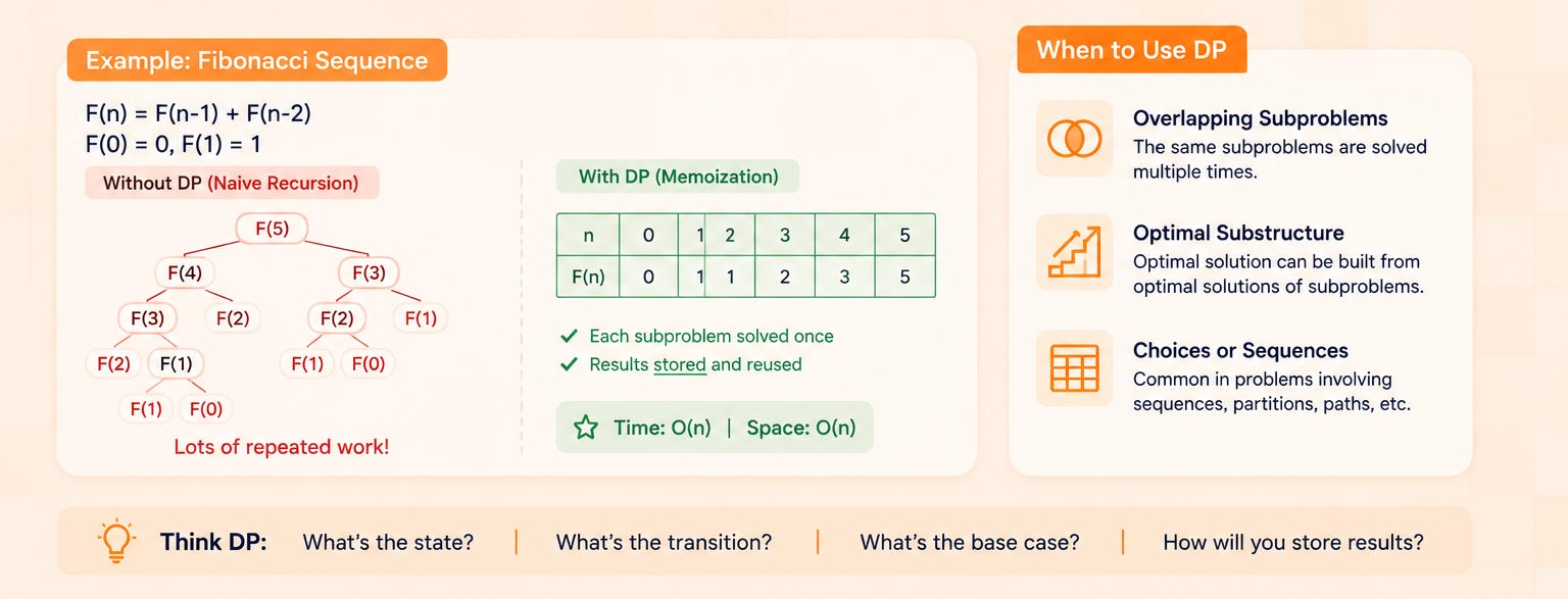
What it is: Break a problem into overlapping subproblems and store their solutions to avoid recomputation. Can be top-down with memoization or bottom-up with a table.
The signal: “Number of ways,” “minimum cost,” “maximum value.” Optimization problems where the answer for input N can be expressed using answers for smaller inputs.
Canonical example: Climbing stairs. You can take 1 or 2 steps at a time. How many distinct ways to reach step N? f(N) = f(N-1) + f(N-2).
What it tests: Whether you can see overlapping subproblem structure in optimization problems.
Pattern 7: Backtracking
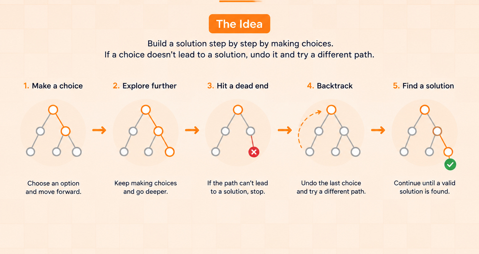
What it is: Build candidate solutions incrementally and abandon (backtrack from) candidates that cannot lead to a valid solution.
The signal: “All permutations,” “all combinations,” “all subsets,” “generate all valid X.”
Canonical example: Generate all permutations of a list. For each position, try each remaining element. Recurse. After recursion, undo the choice.
What it tests: Whether you can systematically explore a solution space without doing extra work on invalid branches.
Pattern 8: Heaps / Priority Queues
What it is: Use a heap data structure to efficiently track the smallest or largest K elements, or to repeatedly process the highest-priority item.
The signal: “Top K,” “smallest K,” “Kth largest,” “median of a stream,” “merge sorted lists.”
Canonical example: Find the Kth largest element. Maintain a min-heap of size K. For each element, if heap is smaller than K, push. Otherwise, if element is larger than heap’s min, pop and push.
What it tests: Whether you recognize that a heap is the right data structure when you need ongoing access to extremes without sorting.
Pattern 9: Linked List Manipulation
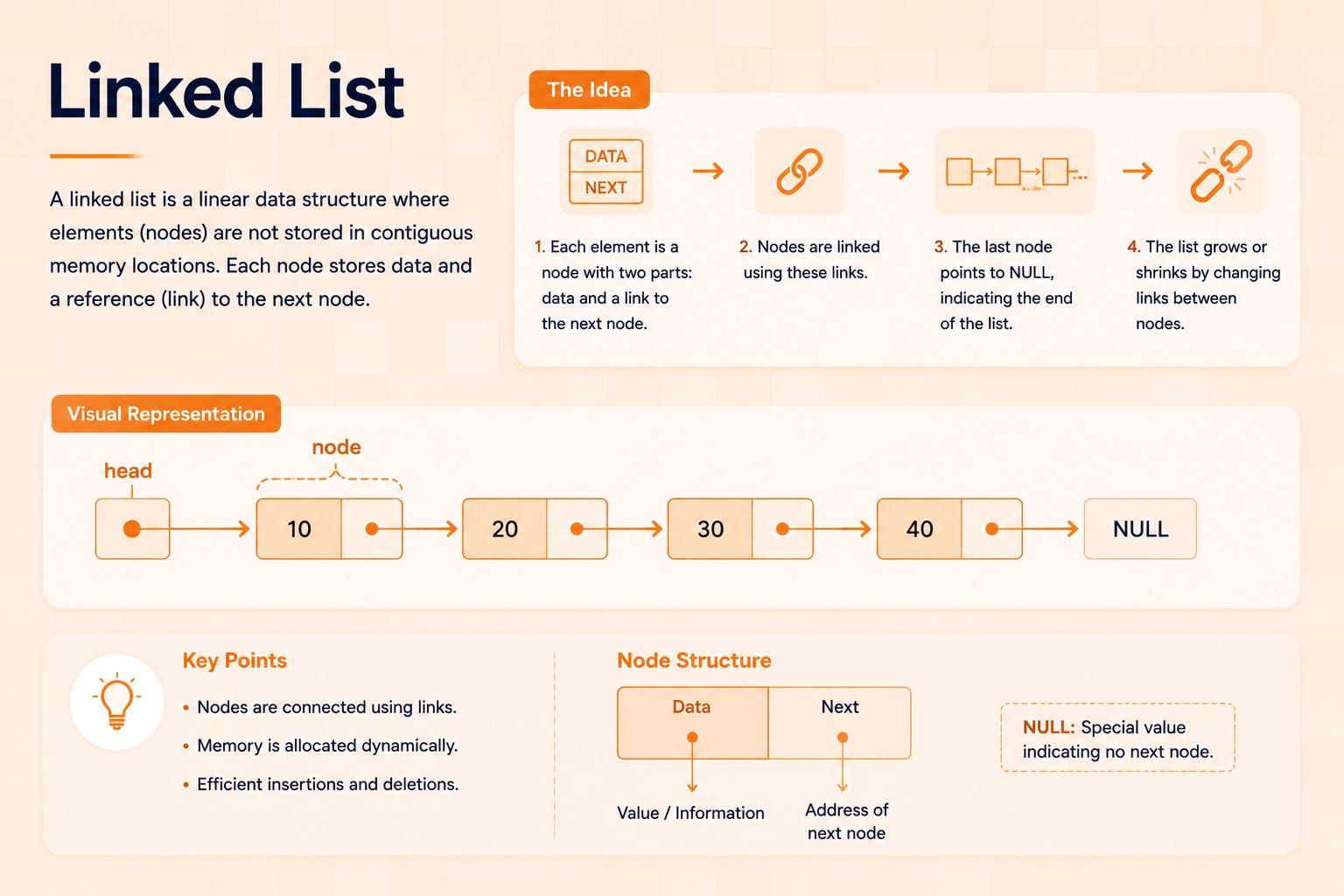
What it is: Modify pointers in a linked list to reverse it, find the middle, detect cycles, or merge two lists.
The signal: Input is a linked list. Words like “reverse,” “merge,” “cycle,” “middle,” “intersection.”
Canonical example: Detect a cycle. Floyd’s algorithm: slow pointer (one step) and fast pointer (two steps). If they meet, cycle exists.
What it tests: Pointer manipulation fluency. New grads who fumble linked list pointers signal rust on fundamentals.
Pattern 10: Stack-Based Problems
What it is: Use a stack to track elements that need processing in last-in-first-out order. Common applications: matching parentheses, evaluating expressions, finding next greater element.
The signal: Matching pairs (parentheses, brackets). “Next greater element.” Expression evaluation. Words like “valid,” “balanced,” “next greater.”
Canonical example: Valid parentheses. Push opening brackets onto a stack. For each closing bracket, pop the stack and check it matches.
What it tests: Whether you recognize when LIFO ordering simplifies a problem.
TIER 3: The Next 5 (Appear Regularly)
Pattern 11: Greedy Algorithms
What it is: Make the locally optimal choice at each step, assuming local optimality leads to global optimality.
The signal: “Maximum X with constraint Y.” Scheduling problems. Interval problems. “Minimum number of operations to...”
Canonical example: Activity selection. Given activities with start and end times, find the maximum number that don’t overlap. Sort by end time, then greedily pick the next activity that starts after the previous one ended.
What it tests: Whether you can identify when greedy local choices yield global optimum (which is not always; backtracking or DP may be needed instead).
Pattern 12: Graph Algorithms (Topological Sort, Union-Find)
What it is: A family of algorithms for directed dependencies (topological sort) or connectivity components (union-find).
The signal: “Prerequisites,” “course schedule,” “task ordering” → topological sort. “Connected components,” “groups,” “is X connected to Y” → union-find.
Canonical example: Course schedule. Given courses with prerequisites, can all be finished? Build directed graph, detect cycles using DFS or Kahn’s algorithm. No cycle = all can be finished.
What it tests: Recognition of when dependency or connectivity structure underlies the problem.
Pattern 13: Trie (Prefix Tree)
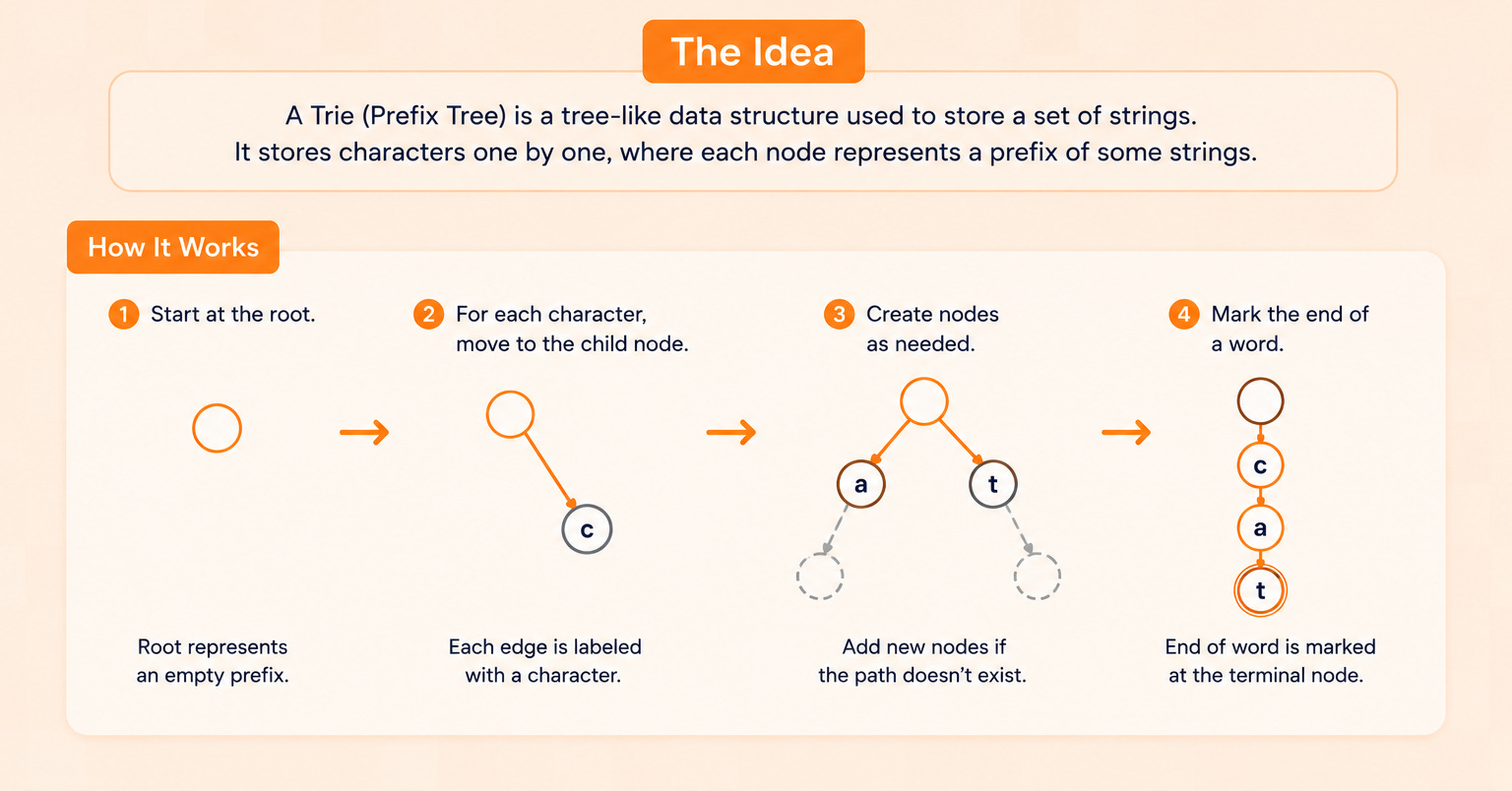
What it is: A tree-like data structure for storing strings where prefixes are shared, enabling O(L) operations for insert and search.
The signal: “Autocomplete,” “prefix matching,” “word search,” “dictionary lookups.”
Canonical example: Implement an autocomplete system. Build a trie from the dictionary. Traverse to the prefix node, return all words below it.
What it tests: Whether you recognize when a prefix-sharing structure beats a hash map for string operations.
Pattern 14: Bit Manipulation
What it is: Solve problems by operating on the binary representation of integers. XOR, bit shifts, bitmasks.
The signal: “Binary,” “XOR,” “single number,” “missing number from 0 to N.” “Set,” “unset,” “toggle bit.”
Canonical example: Find the single number. Given an array where every element appears twice except one, find the unique element. XOR all elements. Pairs cancel out. Result is the unique value.
What it tests: Whether you can recognize when bit-level operations make a problem O(1) space instead of O(n).
Pattern 15: Matrix Traversal
What it is: Walk through a 2D grid using DFS, BFS, or directional iteration. Common applications: islands, paths, flood fill.
The signal: 2D grid as input. “Number of islands,” “shortest path in grid,” “rotting oranges,” “flood fill.”
Canonical example: Number of islands. DFS or BFS from each unvisited land cell, marking visited cells. Increment count for each new search.
What it tests: Whether you can apply graph traversal techniques to grid-shaped problems.
TIER 4: The Last 5 (Less Frequent But Standard)
Pattern 16: Two Heaps
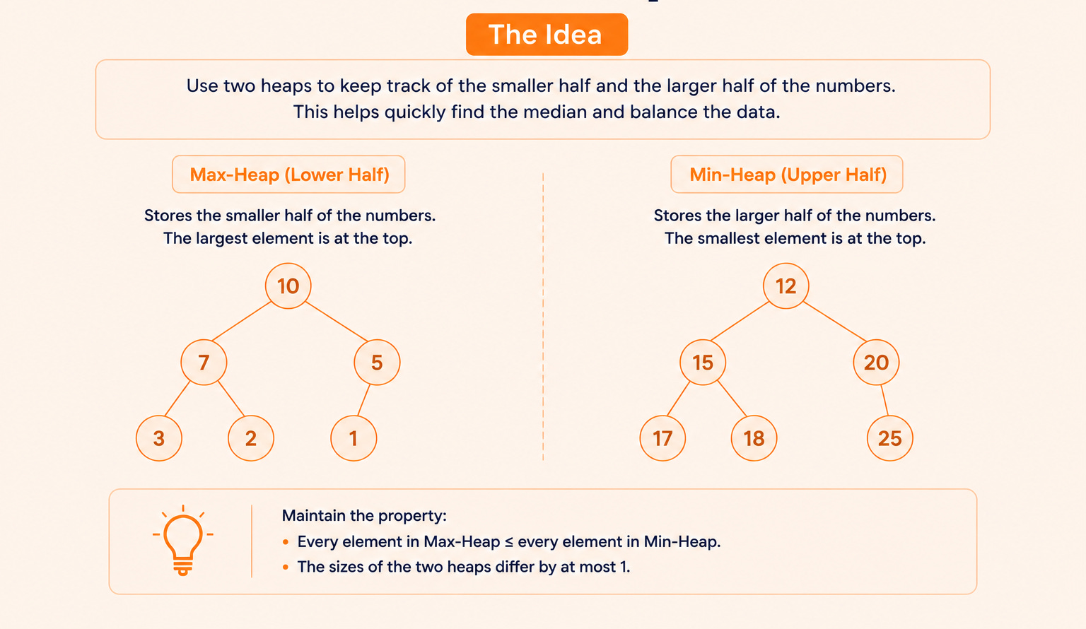
What it is: Maintain two heaps (typically one max-heap and one min-heap) to track elements above and below a running median.
The signal: “Median of a data stream,” “find median in sliding window,” “balance two sets of numbers.”
Canonical example: Median of a data stream. Max-heap for lower half, min-heap for upper half. Median is either the top of one heap or the average of both tops.
What it tests: Whether you can combine multiple data structures to maintain dynamic invariants.
Pattern 17: K-Way Merge
What it is: Merge K sorted lists or sequences efficiently using a heap.
The signal: “Merge K sorted X.” “Kth smallest in K sorted lists.”
Canonical example: Merge K sorted linked lists. Push the head of each list into a min-heap. Pop the smallest, advance that list, push the next element. Continue until heap is empty.
What it tests: Recognition that K independent sorted structures can be combined with a heap-based approach.
Pattern 18: Cyclic Sort
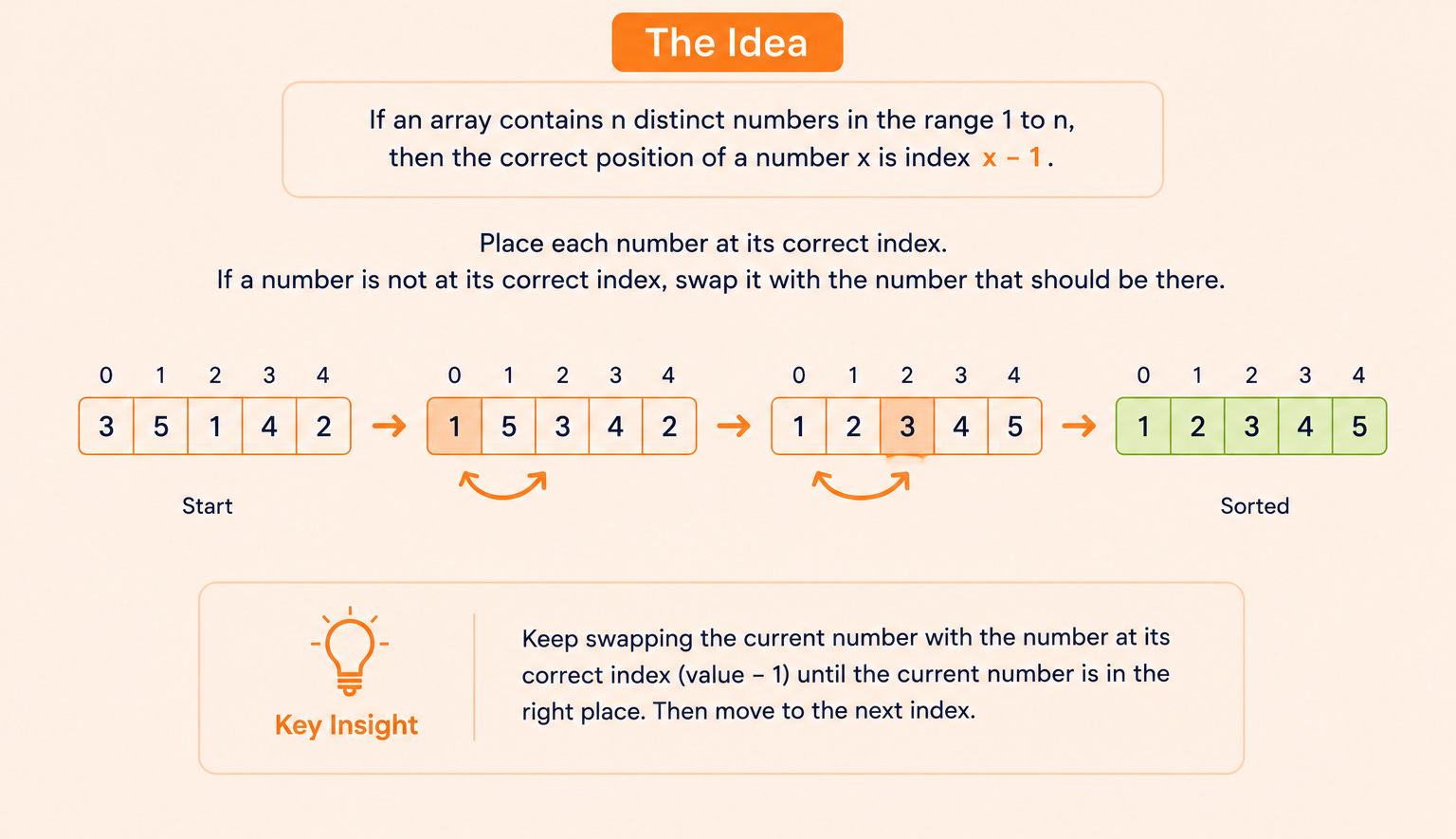
What it is: Sort an array in place by repeatedly placing each element at its correct index, when array contains numbers in a known range (like 0 to N).
The signal: Array contains numbers from a specific range (e.g., 1 to N). “Find the missing number,” “find duplicates.”
Canonical example: Find all numbers missing from an array containing values 1 to N. Place each number at its correct index. The indices that don’t have the correct number indicate missing values.
What it tests: Whether you recognize when in-place sorting can save space.
Pattern 19: Dynamic Programming (Advanced — 2D)
What it is: Extension of DP where the state space is two-dimensional. Common applications: longest common subsequence, edit distance, matrix path problems.
The signal: Problems involving two sequences or 2D grids with optimization. “Longest common subsequence,” “edit distance,” “minimum path sum in a grid.”
Canonical example: Longest common subsequence. Build a 2D table where dp[i][j] is the LCS length of the first i characters of string A and first j characters of string B.
What it tests: Whether you can extend 1D DP thinking to 2D state spaces.
Pattern 20: Shortest Path Algorithms (Dijkstra, Bellman-Ford)
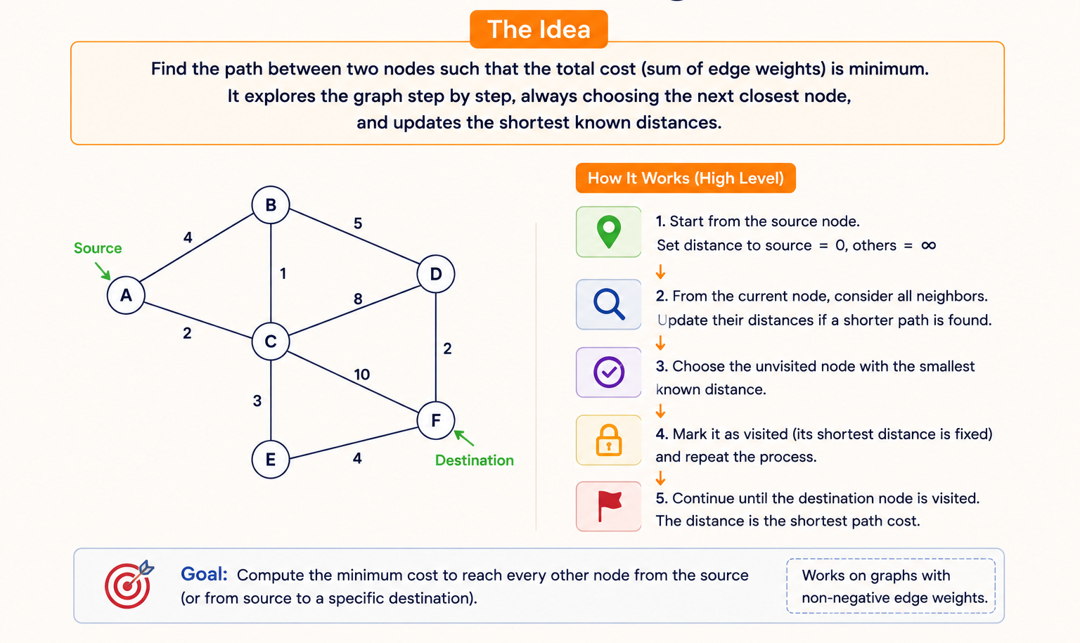
What it is: Find the shortest path in a weighted graph. Dijkstra for non-negative weights. Bellman-Ford for graphs with negative weights.
The signal: Weighted graph. “Shortest distance,” “minimum cost path.”
Canonical example: Cheapest flights with at most K stops. Modified Dijkstra or Bellman-Ford with a stop constraint.
What it tests: Whether you have the algorithmic depth to handle weighted graphs, which is rare for new grads but appears at the higher end of L4 problem difficulty.
How These Patterns Combine
In real interviews, harder problems often combine two or three patterns.
New grad interviews focus mostly on single-pattern problems, with occasional 2-pattern combinations.
Common combinations new grads encounter:
Sliding window + hash map. Longest substring with at most K distinct characters.
Tree traversal + DP. Maximum path sum in a binary tree.
Binary search + greedy. Capacity to ship packages within D days.
DFS + memoization. Most “number of distinct paths” problems on grids with obstacles.
The pattern combinations are not new patterns. They are two patterns from this list, layered together.
If you understand each pattern individually, the combinations come more naturally.
How to Study These Patterns
Three actions to take if you are working through this list during interview prep.
Action 1: Solve 5 to 10 problems per pattern, not 50. Volume per pattern is less important than pattern coverage. A candidate who has solved 10 problems on each of the 20 patterns is better prepared than a candidate who has solved 200 problems all on the top 3 patterns.
Action 2: Annotate each solved problem with the pattern. After solving a problem, write down which pattern (or combination) it used, what the signal in the problem statement was, and what the time and space complexity ended up being. This builds the pattern-recognition reflex.
Action 3: When you encounter a new problem, force yourself to identify the pattern before coding. Even if you are alone. The reflex of pattern recognition under time pressure is what separates candidates who solve unfamiliar problems from candidates who freeze.
The candidates who get FAANG offers in 2026 are not the ones with the most LeetCode problems solved. They are the ones who can pattern-match a new problem within 60 seconds and start solving with confidence.
The 20 patterns above are the alphabet. Solving problems is how you learn to read.