
Backtracking: The “Try, Recurse, Undo” Mental Model
What is backtracking, and how does the try-recurse-undo pattern work? A beginner-friendly explanation with subsets, permutations, and N-Queens examples.

Backtracking has a fearsome reputation.
It shows up in problems that sound hard, generate every possible combination, solve the N-Queens puzzle, find all the ways to partition a string, and the textbook solutions are dense recursive functions that look like magic.
Beginners often decide backtracking is an advanced topic to avoid.
It isn’t.
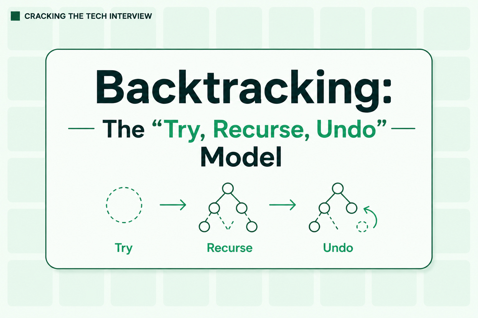
Underneath every backtracking solution is one simple, repeating rhythm: try a choice, recurse to explore the consequences, then undo the choice and try the next one.
Try, recurse, undo.
Once you internalize that three-beat pattern, the scary recursive functions reveal themselves as the same skeleton over and over, and a whole category of “find all the possibilities” problems becomes approachable.
This post explains backtracking through that mental model: what it is, the try-recurse-undo rhythm, worked examples that all share the same skeleton, and how to recognize when a problem wants it.
What Is Backtracking
Backtracking is a way to explore all possible combinations of choices by building them up one decision at a time, and abandoning a path the moment it can’t lead to a valid answer (then “backing up” to try something else).
The mental image that makes it click: you’re exploring a maze of decisions. At each fork, you pick a direction and walk down it.
If it leads somewhere good, great. If it leads to a dead end, you walk back to the fork and try a different direction. You systematically explore every path, but you never waste time continuing down a route you already know is doomed.
That “walk forward, hit a dead end, back up and try the next option” is exactly what backtracking does, and the “back up” is where the name comes from.
The reason it’s recursive is that “explore the consequences of this choice” is itself a smaller version of the same problem.
Make a choice, then solve the rest the same way. That self-similarity is what makes recursion the natural tool.
The three-beat rhythm: try, recurse, undo
Here is the heart of every backtracking solution, the pattern you’ll see again and again:
Try a choice, add it to the partial solution you’re building.
Recurse, explore everything that follows from that choice.
Undo the choice, remove it, so you’re back to a clean state to try the next option.
That undo step is the soul of backtracking and the part beginners most often miss.
After you’ve fully explored what happens when you make a choice, you have to take it back so the next choice starts from the same clean slate.
Without the undo, your choices pile up and contaminate each other.
With it, every branch of the exploration starts fresh.
Here’s the rhythm as a skeleton, in pseudocode:
function backtrack(current_solution):
    if current_solution is complete:
        record it
        return
    for each possible next choice:
        make the choice        # TRY
        backtrack(...)          # RECURSE
        undo the choice         # UNDO
Every backtracking problem is a variation on this.
The differences are just what counts as a choice, when a solution is complete, and whether some choices can be skipped early.
The skeleton stays the same.
Example 1: generating all subsets
The clearest first example.
Given [1, 2, 3], produce every subset: the empty set, [1], [1,2], [1,2,3], [1,3], [2], [2,3], [3].
The choice at each step is “which remaining element do I add next?”
def subsets(nums):
    result = []
    path = []                          # the subset we're building
    def backtrack(start):
        result.append(path[:])         # record the current subset (a copy)
        for i in range(start, len(nums)):
            path.append(nums[i])       # TRY: add this element
            backtrack(i + 1)           # RECURSE: build on it
            path.pop()                 # UNDO: remove it, try the next
    backtrack(0)
    return result

subsets([1, 2, 3])
# -> [[], [1], [1,2], [1,2,3], [1,3], [2], [2,3], [3]]
Watch the three beats: path.append is the try, backtrack(i+1) is the recurse, path.pop() is the undo.
After exploring every subset that includes nums[i], we pop it off so the loop can try the next element with a clean path.
That path.pop() is what lets one path list serve the entire exploration without the choices contaminating each other.
One subtle but important detail: we append path[:], a copy of the current path, not path itself. Because path keeps changing as we backtrack, storing it directly would mean all our recorded subsets point at the same list, which ends up empty.
Copying captures a snapshot.
(This connects directly to mutability, which is worth understanding alongside backtracking.)
Example 2: generating all permutations
Same skeleton, different choice.
A permutation uses all the elements in some order, so the choice is “which unused element comes next?”, and a solution is complete when nothing remains:
def permutations(nums):
    result = []
    def backtrack(path, remaining):
        if not remaining:                       # complete: nothing left
            result.append(path[:])
            return
        for i in range(len(remaining)):
            path.append(remaining[i])           # TRY
            backtrack(path, remaining[:i] + remaining[i+1:])  # RECURSE without it
            path.pop()                          # UNDO

    backtrack([], nums)
    return result

permutations([1, 2, 3])
# -> [[1,2,3], [1,3,2], [2,1,3], [2,3,1], [3,1,2], [3,2,1]]
Identical rhythm: try an element, recurse on what’s left, undo.
The only real difference from subsets is the definition of “complete” (here, no elements remaining) and that each recursion passes along the remaining unused elements.
Notice you’re not learning a new algorithm, you’re reapplying the same skeleton with a different notion of a choice.
Example 3: pruning, where backtracking earns its name
The examples so far explore every combination.
Backtracking’s real power shows when you can abandon a path early because it can’t possibly work, which saves enormous amounts of work. The classic is N-Queens: place N queens on an NxN board so none attack each other.
The choice is where to put the queen in each row; the pruning is skipping any column already under attack:
def solve_n_queens(n):
    count = 0
    cols, diag1, diag2 = set(), set(), set()
    def backtrack(row):
        nonlocal count
        if row == n:                    # placed all n queens: a solution
            count += 1
            return
        for col in range(n):
            if col in cols or (row - col) in diag1 or (row + col) in diag2:
                continue                # PRUNE: this square is attacked, skip it
            cols.add(col); diag1.add(row - col); diag2.add(row + col)   # TRY
            backtrack(row + 1)                                           # RECURSE
            cols.remove(col); diag1.remove(row - col); diag2.remove(row + col)  # UNDO
    backtrack(0)
    return count

solve_n_queens(4)   # -> 2
solve_n_queens(8)   # -> 92
The skeleton is unchanged, try, recurse, undo, but now there’s a fourth idea layered in: prune.
Before trying a choice, check whether it’s even viable, and if not, skip it entirely, never recursing down a doomed path.
This is what makes backtracking dramatically faster than blindly generating every arrangement and checking each at the end.
The earlier you can prune, the more work you save.
Pruning is the difference between backtracking as a clever search and backtracking as glorified brute force.
How to recognize a backtracking problem
The tells are consistent.
Reach for backtracking when a problem asks you to generate or find all the possibilities, all combinations, all subsets, all permutations, all valid arrangements, all ways to do something, especially when each result is built from a sequence of choices and choices may need to be undone to explore alternatives.
Signal words: “all combinations,” “all subsets,” “all permutations,” “every possible,” “find all ways,” “generate all.”
Puzzle-like constraint problems (N-Queens, Sudoku, word search, partitioning) are also classic backtracking, because they involve trying placements and abandoning ones that violate the rules.
One important distinction: if the problem asks for the number of ways or the best way rather than listing every possibility, it might be dynamic programming instead, which counts or optimizes without enumerating each option.
“List all the ways” points to backtracking; “how many ways” or “the maximum value” often points to DP.
The difference is whether you need the possibilities themselves or just a count or optimum over them.
A note on cost
Be honest about complexity: backtracking often explores an exponential number of possibilities, because that’s genuinely how many there are (the number of subsets of n items is 2ⁿ, the number of permutations is n!).
When a problem truly requires generating all of them, that cost is unavoidable, you can’t list 2ⁿ subsets in less than 2ⁿ time.
This is why pruning matters so much: it doesn’t change the worst case, but in practice it can cut away vast portions of the search space, turning an intractable exploration into a feasible one.
And it’s why the constraints matter, a small input bound (like n up to 20 or fewer) is often a hint that an exponential backtracking solution is exactly what’s expected.
Frequently asked questions
What’s the difference between backtracking and plain recursion?
Backtracking is a kind of recursion, with a specific shape: it builds a solution through a sequence of choices and undoes each choice after exploring it, so it can try alternatives. The “undo” step and the systematic exploration of all options are what make it backtracking specifically.
Why is the “undo” step so important?
Because you reuse the same partial-solution structure across the whole exploration. After exploring what happens with a choice made, you must remove it so the next option starts from a clean state. Skip the undo and your choices accumulate and corrupt each other. It’s the most commonly forgotten piece.
When should I use backtracking instead of dynamic programming?
Use backtracking when you need to enumerate actual possibilities (list all subsets, find all valid arrangements). Use DP when you need a count or an optimum and don’t need the possibilities themselves. “List all” means backtracking; “how many” or “best” often means DP.
Why are backtracking solutions often slow?
Because they explore an exponential number of possibilities, and for problems that genuinely ask for all of them, that’s inherent, there are simply that many. Pruning (abandoning doomed paths early) is the key tool to make it practical, and small input limits usually signal that an exponential solution is acceptable.
What is “pruning”?
Skipping a choice that can’t possibly lead to a valid solution, before recursing into it. In N-Queens, you skip a square that’s already attacked. Pruning is what makes backtracking far more efficient than generating every arrangement and filtering at the end.
Why do I need to copy the path when recording a solution?
Because the path keeps changing as you backtrack. If you store the path object directly, all your recorded results point at the same, constantly-changing list. Storing a copy captures a snapshot of that moment. This is a direct consequence of how mutable objects work.
The bottom line
Backtracking is recursion with a three-beat rhythm: try a choice, recurse to explore its consequences, then undo it to try the next option.
That single pattern, plus the idea of pruning doomed paths early, is the engine behind every “generate all possibilities” and constraint-puzzle problem, from subsets and permutations to N-Queens.
The scary-looking recursive functions are all the same skeleton with different definitions of “a choice” and “a complete solution.”
Recognize the tells, “all combinations,” “every possible,” “find all ways”, reach for the try-recurse-undo skeleton, prune whenever you can, and remember to undo each choice and to copy your solutions when you record them.
Do that, and a topic that looks like advanced wizardry turns out to be one repeating, learnable rhythm.