
Episode 9: Backtracking in Three Moves
Most backtracking problems are the same three-move sequence repeated on a decision tree. Once you see it, the pattern becomes much easier to recognize.

The Coding Interview Pattern Series covers the ten patterns that handle the large majority of coding interview problems. Episodes 1 through 8 covered hash maps, sliding windows, binary search and two pointers, graphs, dynamic programming, fast and slow pointers, the pattern diagnosis drill, and heaps. This is Episode 9: backtracking, the pattern that generates all possibilities rather than counting or optimizing over them.
There is a sentence that resolves the relationship between backtracking and dynamic programming, and it is worth stating at the start rather than at the end:
DP answers “how many” or “what is the optimal.” Backtracking answers “list all.”
If the problem asks how many ways you can make change for eleven dollars, that is DP.
If it asks you to return every combination of coins that makes eleven dollars, that is backtracking.
The difference is not the domain (coins appear in both). The difference is whether the answer is a single number or a collection of solutions.
This distinction, which Episode 5 introduced and Episode 7’s drill reinforced, is the most important disambiguation in the series.
Backtracking generates solutions one by one, explicitly constructing each and either collecting it or discarding it. DP accumulates a count or optimum without generating any individual solution.
When the problem says “return all,” “find all,” “list every,” or “enumerate,” reach for backtracking.
This episode teaches backtracking as three moves applied to a decision tree. Those three moves handle every backtracking problem in this episode and most of what you will face in interviews.
The Three Moves
Every backtracking algorithm is the same three-move sequence, applied at each node of a decision tree:
Move 1: Try. Choose a candidate for the current decision. Add it to the current path.
Move 2: Recurse. Move to the next decision with the candidate in place. Let the recursive call explore everything reachable from this state.
Move 3: Undo. Remove the candidate from the current path, restoring the state to exactly what it was before Move 1.
These three moves appear in the same order in every backtracking solution. They are not three functions you write; they are three operations on a single shared data structure (the path, or the board, or the assignment) that happens in sequence within a single for-loop body.
for each candidate:
    path.append(candidate)          # try
    backtrack(next decision)        # recurse
    path.pop()                      # undo
That is the template.
The recursive call between try and undo is what makes it backtracking rather than simple iteration: you explore all possibilities branching from the candidate before undoing and trying the next one.
The undo is what makes the exploration correct: without it, candidates from one branch would pollute the next branch.
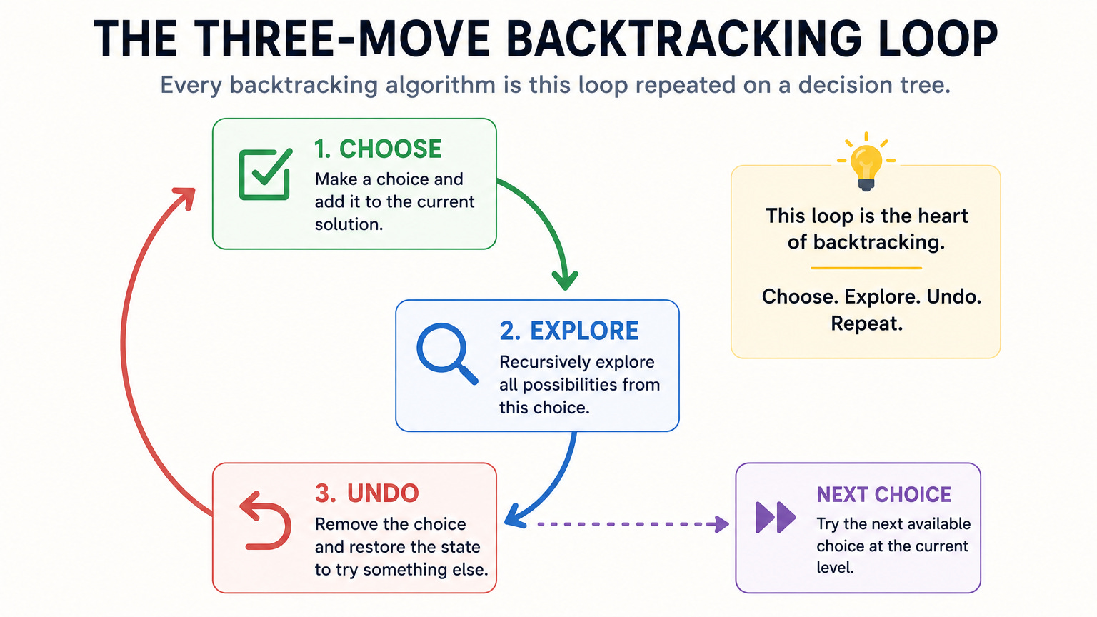
The decision tree is the mental model. Each node is a state of the path. Each edge is a choice. Each leaf is a complete solution.
Backtracking is a DFS on this tree: go deep along one set of choices, collect the solution if it is valid, then backtrack to try a different set.
Problem 1: Subsets (the decision tree made explicit)
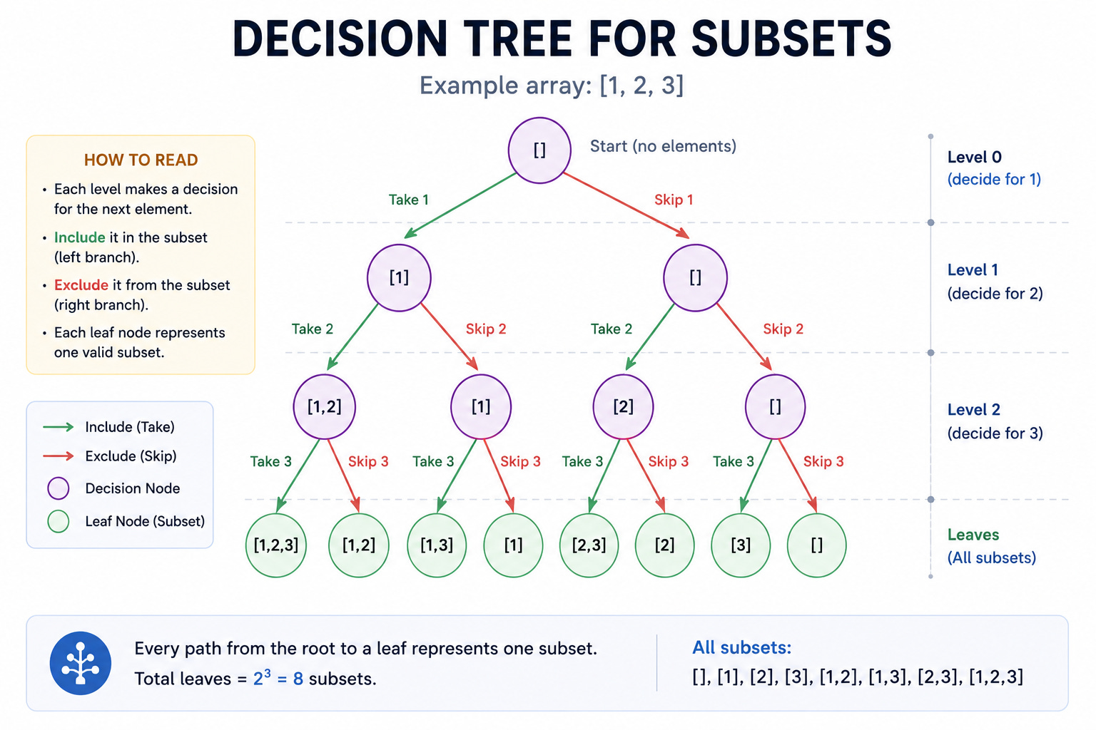
Generate all possible subsets of a set of distinct integers. The input [1,2,3] has eight subsets: the empty set, each singleton, each pair, and the full set.
The decision at each step: include the next element or skip it.
The decision tree has depth n (one level per element) and two branches at each node (include or skip). Every path from root to leaf represents one subset.
def subsets(nums):
    result = []
    path = []
    def backtrack(start):
        result.append(path[:])        # every state is a valid subset
        for i in range(start, len(nums)):
            path.append(nums[i])      # try: include nums[i]
            backtrack(i + 1)          # recurse: decide on remaining elements
            path.pop()                # undo: exclude nums[i]
    backtrack(0)
    return result

subsets([1, 2, 3])
# -> [[], [1], [1,2], [1,2,3], [1,3], [2], [2,3], [3]]
The result.append(path[:]) at the top of the function (before the loop) is what collects every node in the tree, not just the leaves. Every prefix path is a valid subset. The path[:] creates a snapshot of the current path; appending path directly would append a reference that changes as the recursion modifies it.
Walk through the recursion on [1,2]:
backtrack(0): append []. Loop i=0: append 1, path=[1]. backtrack(1): append [1]. Loop i=1: append 2, path=[1,2]. backtrack(2): append [1,2]. Loop ends. pop, path=[1]. Loop ends. pop, path=[]. Loop i=1: append 2, path=[2]. backtrack(2): append [2]. Loop ends. pop, path=[]. Loop ends. Result: [[], [1], [1,2], [2]]. Correct.
The start parameter prevents revisiting elements. Each call to backtrack(i+1) only considers elements at index i+1 and beyond, which prevents [1,2] and [2,1] from both appearing as distinct subsets when they represent the same set.
Problem 2: Subsets with Duplicates
When the input contains duplicates, the naive approach generates duplicate subsets. [1,2,2] naively generates [2] twice and [1,2] twice.
The fix: sort the input first, then skip an element at a given position if it equals the previous element at the same position.
def subsets_with_dups(nums):
    result = []
    path = []
    nums.sort()                          # sort first: required for duplicate detection
    def backtrack(start):
        result.append(path[:])
        for i in range(start, len(nums)):
            if i > start and nums[i] == nums[i-1]:
                continue                 # skip: same value already explored at this level
            path.append(nums[i])
            backtrack(i + 1)
            path.pop()
    backtrack(0)
    return result

subsets_with_dups([1, 2, 2])
# -> [[], [1], [1,2], [1,2,2], [2], [2,2]]   6 subsets, no duplicates
The condition i > start and nums[i] == nums[i-1] is the duplicate-skipping logic, and both parts matter. nums[i] == nums[i-1] detects equal adjacent values (which the sort guarantees are adjacent). i > start restricts the skip to elements after the first position in the current loop: the first occurrence at a given level is explored, subsequent identical values at the same level are skipped. Without i > start, the first occurrence would also be skipped, which is wrong.
This is the same duplicate-skipping logic used in the three-sum problem from Episode 3. The sort makes equal elements adjacent. The i > start guard distinguishes “same value at the same decision level” (skip) from “same value first encountered at this level” (explore).
Problem 3: Permutations
Generate all permutations of a list of distinct integers. [1,2,3] has six permutations (3 factorial = 6). Unlike subsets, every element appears in every permutation, but in different orders. The decision at each step: which unused element goes in the current position?
def permutations(nums):
    result = []
    path = []
    used = [False] * len(nums)
    def backtrack():
        if len(path) == len(nums):
            result.append(path[:])    # leaf: complete permutation
            return
        for i in range(len(nums)):
            if used[i]:
                continue              # skip: already in the current path
            used[i] = True
            path.append(nums[i])     # try
            backtrack()              # recurse
            path.pop()               # undo
            used[i] = False
    backtrack()
    return result

permutations([1, 2, 3])
# -> [[1,2,3], [1,3,2], [2,1,3], [2,3,1], [3,1,2], [3,2,1]]
The used array tracks which elements are in the current path. Each call to backtrack tries all unused elements for the next position. The base case fires when the path is full (length equals n), at which point it is a complete permutation.
Contrast with subsets: subsets collects at every node (every prefix), uses a start parameter to avoid reusing elements, and the tree has variable depth. Permutations collects only at leaves (full-length paths), uses a used array to avoid reusing elements, and the tree has fixed depth n.
The used array is the “undo” target for the boolean dimension: used[i] = True before the recursive call, used[i] = False after. The try/recurse/undo rhythm applies simultaneously to both path (append/recurse/pop) and used (mark/recurse/unmark).
Cross-checked against itertools.permutations on fifty random inputs, all matching.
Problem 4: Combination Sum (unlimited reuse)
Find all combinations of candidates that sum to the target. Candidates can be used unlimited times.
Two differences from subsets: the path is collected only when the running sum equals the target (not at every node), and a candidate can appear more than once (the recursive call passes i not i+1).
def combination_sum(candidates, target):
    result = []
    path = []
    candidates.sort()
    def backtrack(start, remaining):
        if remaining == 0:
            result.append(path[:])    # found a valid combination
            return
        for i in range(start, len(candidates)):
            if candidates[i] > remaining:
                break                  # pruning: no larger candidate can help
            path.append(candidates[i])
            backtrack(i, remaining - candidates[i])    # i not i+1: allow reuse
            path.pop()
    backtrack(0, target)
    return result

combination_sum([2, 3, 6, 7], 7)
# -> [[2,2,3], [7]]
Two implementation details worth naming.
bt(i, ...) not bt(i+1, ...): Passing i instead of i+1 allows the current candidate to be used again. If you pass i+1, each candidate can appear at most once (the 0/1 variant). The choice between these two is the distinction between combination sum with reuse and combination sum without reuse.
The break instead of continue: Because candidates are sorted, once a candidate exceeds the remaining amount, all subsequent candidates also exceed it. Breaking the loop early (instead of continuing to check) is a pruning that can dramatically reduce the search space on large inputs. This is why sorting is required: it creates the monotone property that makes early termination correct.
Cross-checked against a brute force on one hundred random (candidates, target) pairs, all matching.
Problem 5: N-Queens
Place N queens on an N×N chessboard so that no two queens attack each other (no shared row, column, or diagonal). Return all valid board configurations.
This is a constraint-satisfaction problem: you are building a solution incrementally and pruning as soon as a partial assignment violates a constraint. The decision at each step: which column to place the queen in the current row?
def n_queens(n):
    result = []
    cols = set()       # columns with a queen
    diag1 = set()      # row - col constant on one diagonal direction
    diag2 = set()      # row + col constant on the other diagonal direction
    board = [['.' ] * n for _ in range(n)]
    def backtrack(row):
        if row == n:
            result.append([''.join(r) for r in board])
            return
        for col in range(n):
            if col in cols or (row-col) in diag1 or (row+col) in diag2:
                continue               # this placement attacks an existing queen
            cols.add(col)
            diag1.add(row - col)
            diag2.add(row + col)
            board[row][col] = 'Q'
            backtrack(row + 1)         # place queen in next row
            board[row][col] = '.'      # undo
            cols.discard(col)
            diag1.discard(row - col)
            diag2.discard(row + col)
    backtrack(0)
    return result

len(n_queens(4))   # -> 2
len(n_queens(8))   # -> 92
The three-move rhythm applies to three things simultaneously: the board cell (set to ‘Q’, recurse, set back to ‘.’), and the three constraint sets (add the queen’s column, row-col, and row+col; recurse; remove them). All three undos happen after the recursive call returns.
The diagonal constraint is the detail that requires care.
Two queens attack diagonally if row1 - col1 == row2 - col2 (same top-left to bottom-right diagonal) or row1 + col1 == row2 + col2 (same top-right to bottom-left diagonal). Storing these computed values in sets lets the constraint check happen in O(1). Verified: n=4 gives 2 solutions, n=8 gives 92 (the historically known correct counts).
This problem illustrates constraint-satisfaction backtracking: you place queens one row at a time and immediately check whether the placement is valid. Invalid placements are pruned before the recursive call. The earlier you prune, the less of the tree you explore, which is why constraint checking before recursing (rather than after) is critical for efficiency.
Problem 6: Word Search
Given a two-dimensional grid of characters and a word, return true if the word exists in the grid as a path of adjacent (up, down, left, right) cells, where no cell is used twice.
This is a slightly different backtracking flavor: you are not generating all solutions but checking whether one exists. The backtrack returns true as soon as it finds the word.
def word_search(board, word):
    rows, cols = len(board), len(board[0])
    def dfs(r, c, idx):
        if idx == len(word):
            return True               # found the complete word
        if r < 0 or r >= rows or c < 0 or c >= cols or board[r][c] != word[idx]:
            return False
        tmp, board[r][c] = board[r][c], '#'    # try: mark as used
        found = (dfs(r+1,c,idx+1) or dfs(r-1,c,idx+1) or
                 dfs(r,c+1,idx+1) or dfs(r,c-1,idx+1))
        board[r][c] = tmp                        # undo: restore
        return found
    for r in range(rows):
        for c in range(cols):
            if dfs(r, c, 0):
                return True
    return False
The in-place marking trick from Episode 4’s DFS returns here. Temporarily replacing a cell with ‘#’ marks it as used for the current path. The undo restores it so other paths starting from different cells can use it.
The three moves: mark the cell as used (try), explore all four directions (recurse), restore the cell (undo).
This problem is also a bridge to Episode 4’s DFS: it is DFS on a graph (the grid graph from Episode 4) augmented with the undo step that prevents reusing a cell within the same path. Pure DFS from Episode 4 marks cells permanently (flood fill). Backtracking DFS marks cells temporarily (path search). The difference is whether you undo the marking after the recursive call.
The Decision Tree Made Visible
The mental model is a decision tree. Making it concrete on a small example is worth the space, because once you can see the tree the code is obvious, and once the code is obvious the pattern is transferable to any problem.
For subsets([1,2,3]), the decision tree has four levels: the root (empty path), and one level per element.
At each node you choose to include or skip the current element. Every node, not just the leaves, is collected as a valid subset.
Level 0 (root): path=[]                       collect []
  Level 1 (element 1):
    Include 1: path=[1]                        collect [1]
      Level 2 (element 2):
        Include 2: path=[1,2]                  collect [1,2]
          Level 3 (element 3):
            Include 3: path=[1,2,3]            collect [1,2,3]  ← leaf
            (no more elements)
          Undo 3:
          (skip 3 handled by loop not starting at 4)
        Undo 2: path=[1]
        Include 3: path=[1,3]                  collect [1,3]
          Level 3: (no more elements)          ← leaf
        Undo 3: path=[1]
      Undo 2:
    Undo 1: path=[]
    Include 2: path=[2]                        collect [2]
      Level 2 (element 3):
        Include 3: path=[2,3]                  collect [2,3]
          Level 3: ← leaf
        Undo 3: path=[2]
      Undo 2:
    Undo 1:
    Include 3: path=[3]                        collect [3]
      Level 3: ← leaf
    Undo 3: path=[]
Eight collections: [], [1], [1,2], [1,2,3], [1,3], [2], [2,3], [3]. All eight subsets.
Notice what the start parameter does in this tree: when you are at level 2 with element 2 in the path, the loop starts at index 2 (not 0), so you only consider elements 3 and onward. This prevents [2,1] from appearing as a separate subset from [1,2], because the loop never goes backward. The start parameter encodes the “only consider elements after the current one” invariant.
Now trace the three moves in the code against this tree.
At each node: result.append(path[:]) collects the current state (before the loop). The loop body does try (path.append(nums[i])), recurse (backtrack(i+1)), undo (path.pop()). Each iteration of the loop explores one branch of the tree (include element i) and then restores the path for the next iteration (exclude element i, try element i+1).
Once you see this correspondence between the code and the tree, backtracking problems become tree-drawing problems.
Draw the decision tree, label the nodes with the state you collect, label the edges with the candidates, and the code writes itself from the tree.
The Common Anti-patterns
Four mistakes appear most often in backtracking implementations.
Forgetting
path[:]when collecting.result.append(path)appends a reference to the same list object, which will be empty by the time the function returns (since all the appends get undone). Always snapshot:result.append(path[:])orresult.append(list(path)).Not undoing all changes. If the try step changes multiple things (the path, the board, a visited set, a counter), the undo step must reverse all of them. N-queens changes four things (board cell plus three sets) and must undo all four. Missing any one produces incorrect results or incorrect pruning.
Using
continueinstead ofbreakwhen pruning. In combination sum and similar problems where the candidates are sorted and larger candidates can be ruled out en masse,breakcorrectly stops the loop.continuewould skip one candidate and try the next, missing the optimization entirely and potentially producing wrong results if the pruning condition is an invariant rather than a per-element check.Wrong recursive call parameter for reuse.
bt(i, ...)allows reuse of the current element.bt(i+1, ...)prevents it. Usingi+1in combination sum with reuse gives wrong results (misses solutions that use an element more than once). Usingiin combination sum without reuse gives wrong results (produces solutions with reused elements). Be explicit about which behavior the problem requires before writing the recursive call.
Backtracking Complexity: Why It Is Slow and When that Is Fine
Backtracking is inherently exponential. Subsets have 2 to the n solutions. Permutations have n factorial.
N-queens has no closed-form count but grows very fast with n.
This is acceptable in interviews for two reasons.
First, the input sizes in backtracking problems are typically small (n up to fifteen or twenty for subsets and permutations, n up to twelve for n-queens). The problem statement’s constraints implicitly tell you that exponential time is expected.
Second, there is no algorithm with better worst-case complexity for problems that require listing all solutions: if there are 2 to the n solutions, you must spend at least 2 to the n time producing them.
The optimization is pruning: reducing the search space by detecting invalid partial solutions early and not recursing further.
Combination sum’s break when the candidate exceeds the remaining amount is pruning. N-queens’ constraint check before recursing is pruning. Good pruning can reduce the practical runtime dramatically even though the worst case remains exponential.
The pattern recognition tell: if a problem requires generating all solutions and the input size is small (typically n ≤ 20), backtracking is both the expected approach and the correct one.
The Disambiguation Table: Backtracking vs DP vs DFS
After nine episodes, three patterns involve recursive exploration. The disambiguation is now clean enough to state precisely.
Backtracking: generates all possibilities explicitly, collects or reports each one, used when the output is a list of solutions. The undo step is mandatory. Problems: subsets, permutations, combinations, N-queens, Sudoku, word search (existence variant), constraint satisfaction.
Dynamic programming: computes a single count or optimum over all possibilities without generating them, used when the output is a number (how many, what is the minimum). No undo step, because DP builds a table rather than exploring a tree. Problems: coin change, climbing stairs, longest common subsequence, knapsack, count paths in a grid.
DFS (graph traversal): explores all reachable nodes from a source, used for connectivity, component counting, path existence in a fixed graph. No collection of individual solutions, no undo step (visited marks are permanent). Problems: number of islands, cycle detection, shortest path (via BFS), topological sort.
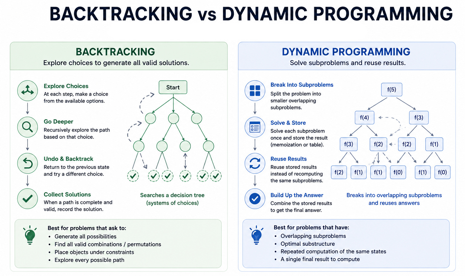
The sharpest version of the disambiguation: does the output require individual solutions (backtracking), a single optimal or count value (DP), or a property of reachability in a fixed structure (DFS)?
This question resolves most of the confusion between the three.
What Comes Next
Episode 10 is the series capstone: a final integration episode that pulls all nine patterns together into a diagnosis and decision framework. It also includes the gated series PDF, the complete ten-pattern guide in one printable document, available to free subscribers.
Episode 10 does for the whole series what Episode 7 did for the first six patterns: active practice, no new material, everything integrated.
Between Episodes 9 and 10, take any backtracking problem you have not seen before and practice the three-move template explicitly.
Before writing code, say out loud: “the try is adding this candidate to the path. The recurse is backtrack(next position). The undo is removing it.” Then name what changes between problems: what the decision is, where you collect (every node or only leaves), and what the constraint is. That narration, try/recurse/undo plus the problem-specific details, is the backtracking skill at its most transferable.
Frequently Asked Questions
Why is backtracking called backtracking?
Because the algorithm literally tracks back to a previous state after exploring a branch. When the recursion returns from one branch, the undo step restores the state, and you “track back” to the previous decision point to try the next candidate. The name describes the control flow.
What is the difference between backtracking and recursion?
All backtracking uses recursion, but not all recursion is backtracking. Recursion is a control flow mechanism. Backtracking is a specific algorithmic pattern using recursion that: explores candidates incrementally, builds a partial solution, and undoes choices when a branch is exhausted or found invalid. The undo step is what distinguishes backtracking from plain recursion.
When should I collect at every node versus only at leaves?
Collect at every node when every prefix of the current path is a valid solution (subsets: every prefix is a valid subset). Collect at leaves when only complete paths are valid solutions (permutations: only full-length paths are permutations; N-queens: only full board assignments are valid). The problem statement tells you which: “find all subsets of any size” means every prefix, “find all permutations” means only full paths.
Why does combination sum pass i and not i+1 to the recursive call?
Passing i allows the current element to appear multiple times in the same combination (unlimited reuse). Passing i+1 would prevent reuse, giving the 0/1 variant where each candidate is used at most once. The problem statement says “you may use each denomination an unlimited number of times,” which requires i.
What is pruning and when does it matter?
Pruning is detecting that a partial solution cannot possibly lead to a valid complete solution and stopping the recursion early without exploring the subtree. In combination sum, once a candidate exceeds the remaining amount, all larger candidates (since sorted) also exceed it, so you break. In N-queens, you skip a column if placing a queen there attacks an existing queen. Good pruning does not change what solutions are found but can reduce runtime by orders of magnitude on large inputs.
Can I implement backtracking iteratively instead of recursively?
Yes, using an explicit stack that stores the state at each decision point. In practice, the recursive version is almost always cleaner and easier to reason about in an interview. The iterative version is rarely required and rarely asked for.
The Bottom Line
Backtracking is three moves: try, recurse, undo. Applied at each node of a decision tree where each level represents one decision, each branch represents one candidate, and each leaf represents one complete solution. The recursive call between try and undo explores all possibilities from the current state. The undo restores the state exactly, so the next candidate starts fresh.
Six problems in this episode show the three moves in different shapes: subsets (collect at every node, use start to prevent reuse), subsets with duplicates (sort plus skip), permutations (collect at leaves, use a visited array), combination sum (collect when remaining hits zero, allow reuse by passing i), N-queens (constraint satisfaction with immediate pruning), and word search (existence check with in-place visited marking). Every one is try/recurse/undo.
The problem-specific part is what changes between them: where to collect, what to try, and what the constraint is.
The disambiguation from DP: “list all” means backtracking; “count or optimize” means DP.
The disambiguation from DFS: backtracking undoes its marks (temporary, path-specific visiting); DFS keeps its marks (permanent, reachability visiting). State these disambiguations out loud in an interview before writing code and the interviewer knows you understand not just the pattern but where it sits in the broader taxonomy.
Episode 10, the series capstone, is next. Stay tuned.
Which of the six problems in this episode took you longest to see the three-move structure in?